pacman::p_load(tmap, sf, tidyverse, knitr)In-class Exercise 1
Tasks
The specific task of this in-class exercise are as follows:
to import Passenger Volume by Origin Destination Bus Stops data set downloaded from LTA DataMall in to RStudio environment,
to import geospatial data in ESRI shapefile format into sf data frame format,
to perform data wrangling by using appropriate functions from tidyverse and sf pakcges, and
to visualise the distribution of passenger trip by using tmap methods and functions.
Getting started
The code chunk below uses p_load() of pacman package to check if the required packages have been installed on the computer. If they are, the packages will be launched. The packages used are:
tmap: for thematic mapping
sf: for geospatial data wrangling
tidyverse: for non-spatial data wrangling
Import Passenger Volume by Origin-Destination Bus Stops
The code chunk below uses the read_csv() function of readr package to import the csv file into R and save it as a R dataframe called odbus.
odbus <- read_csv("data/aspatial/origin_destination_bus_202308.csv")A quick check of odbus tibble data frame shows that the values in OROGIN_PT_CODE and DESTINATON_PT_CODE are in numeric data type.
glimpse(odbus)Rows: 5,709,512
Columns: 7
$ YEAR_MONTH <chr> "2023-08", "2023-08", "2023-08", "2023-08", "2023-…
$ DAY_TYPE <chr> "WEEKDAY", "WEEKENDS/HOLIDAY", "WEEKENDS/HOLIDAY",…
$ TIME_PER_HOUR <dbl> 16, 16, 14, 14, 17, 17, 17, 17, 7, 17, 14, 10, 10,…
$ PT_TYPE <chr> "BUS", "BUS", "BUS", "BUS", "BUS", "BUS", "BUS", "…
$ ORIGIN_PT_CODE <chr> "04168", "04168", "80119", "80119", "44069", "4406…
$ DESTINATION_PT_CODE <chr> "10051", "10051", "90079", "90079", "17229", "1722…
$ TOTAL_TRIPS <dbl> 7, 2, 3, 10, 5, 4, 3, 22, 3, 3, 7, 1, 3, 1, 3, 1, …ORIGIN_PT_CODE and DESTINATION_PT_CODE are numeric variables that are categorical in nature. As such, they should be transformed to factor so that R treats them as a grouping variable.
odbus$ORIGIN_PT_CODE <- as.factor(odbus$ORIGIN_PT_CODE)
odbus$DESTINATION_PT_CODE <- as.factor(odbus$DESTINATION_PT_CODE)
Notice that both of them are in factor data type now.
glimpse(odbus)Rows: 5,709,512
Columns: 7
$ YEAR_MONTH <chr> "2023-08", "2023-08", "2023-08", "2023-08", "2023-…
$ DAY_TYPE <chr> "WEEKDAY", "WEEKENDS/HOLIDAY", "WEEKENDS/HOLIDAY",…
$ TIME_PER_HOUR <dbl> 16, 16, 14, 14, 17, 17, 17, 17, 7, 17, 14, 10, 10,…
$ PT_TYPE <chr> "BUS", "BUS", "BUS", "BUS", "BUS", "BUS", "BUS", "…
$ ORIGIN_PT_CODE <fct> 04168, 04168, 80119, 80119, 44069, 44069, 20281, 2…
$ DESTINATION_PT_CODE <fct> 10051, 10051, 90079, 90079, 17229, 17229, 20141, 2…
$ TOTAL_TRIPS <dbl> 7, 2, 3, 10, 5, 4, 3, 22, 3, 3, 7, 1, 3, 1, 3, 1, …Extract Commuting Flow data
The code chunk below extracts commuting flows on weekday during the rush hour (7am to 9am).
origin7_9 <- odbus %>%
  filter(DAY_TYPE == "WEEKDAY") %>%
  filter(TIME_PER_HOUR >= 7 &
           TIME_PER_HOUR <= 9) %>%
  group_by(ORIGIN_PT_CODE) %>%
  summarise(TRIPS = sum(TOTAL_TRIPS))
It should look similar to the data table below.
kable(head(origin7_9))| ORIGIN_PT_CODE | TRIPS |
|---|---|
| 01012 | 1617 |
| 01013 | 813 |
| 01019 | 1620 |
| 01029 | 2383 |
| 01039 | 2727 |
| 01059 | 1415 |
We will save the output in rds format for future used.
write_rds(origin7_9, "data/rds/origin7_9.rds")The code chunk below will be used to import the save origin7_9.rds into R environment.
origin7_9 <- read_rds("data/rds/origin7_9.rds")Working with Geospatial Data
Geospatial data is adopted to enrich analysis.
Import Bus Stop Locations
The code chunk below uses the st_read() function of sf package to import BusStop shapefile into R as a simple feature data frame called BusStop. As BusStop uses svy21 projected coordinate system, the crs is set to 3414.
busstop <- st_read(dsn = "data/geospatial",
                   layer = "BusStop") %>%
  st_transform(crs = 3414)
Reading layer `BusStop' from data source
`D:\KathyChiu77\ISSS624\In-class Ex\In-class Ex1\data\geospatial'
using driver `ESRI Shapefile'
Simple feature collection with 5161 features and 3 fields
Geometry type: POINT
Dimension: XY
Bounding box: xmin: 3970.122 ymin: 26482.1 xmax: 48284.56 ymax: 52983.82
Projected CRS: SVY21The structure of busstop sf tibble data frame should look as below.
glimpse(busstop)Rows: 5,161
Columns: 4
$ BUS_STOP_N <chr> "22069", "32071", "44331", "96081", "11561", "66191", "2338…
$ BUS_ROOF_N <chr> "B06", "B23", "B01", "B05", "B05", "B03", "B02A", "B02", "B…
$ LOC_DESC <chr> "OPP CEVA LOGISTICS", "AFT TRACK 13", "BLK 239", "GRACE IND…
$ geometry <POINT [m]> POINT (13576.31 32883.65), POINT (13228.59 44206.38),…Import Planning Subzone data
The code chunk below uses the st_read() function of sf package to import MPSZ-2019 shapefile into R as a simple feature data frame called mpsz. To ensure we can use mpsz together with BusStop, mpsz is reprojected to the svy21 projected coordinate system (crs=3413).
mpsz <- st_read(dsn = "data/geospatial",
                   layer = "MPSZ-2019") %>%
  st_transform(crs = 3414)
Reading layer `MPSZ-2019' from data source
`D:\KathyChiu77\ISSS624\In-class Ex\In-class Ex1\data\geospatial'
using driver `ESRI Shapefile'
Simple feature collection with 332 features and 6 fields
Geometry type: MULTIPOLYGON
Dimension: XY
Bounding box: xmin: 103.6057 ymin: 1.158699 xmax: 104.0885 ymax: 1.470775
Geodetic CRS: WGS 84The structure of mpsz sf tibble data frame should look as below.
glimpse(mpsz)Rows: 332
Columns: 7
$ SUBZONE_N <chr> "MARINA EAST", "INSTITUTION HILL", "ROBERTSON QUAY", "JURON…
$ SUBZONE_C <chr> "MESZ01", "RVSZ05", "SRSZ01", "WISZ01", "MUSZ02", "MPSZ05",…
$ PLN_AREA_N <chr> "MARINA EAST", "RIVER VALLEY", "SINGAPORE RIVER", "WESTERN …
$ PLN_AREA_C <chr> "ME", "RV", "SR", "WI", "MU", "MP", "WI", "WI", "SI", "SI",…
$ REGION_N <chr> "CENTRAL REGION", "CENTRAL REGION", "CENTRAL REGION", "WEST…
$ REGION_C <chr> "CR", "CR", "CR", "WR", "CR", "CR", "WR", "WR", "CR", "CR",…
$ geometry <MULTIPOLYGON [m]> MULTIPOLYGON (((33222.98 29..., MULTIPOLYGON (…Geospatial data wrangling
Combining Busstop and mpsz
Code chunk below populates the planning subzone code (i.e. SUBZONE_C) of mpsz sf data frame into busstop sf data frame.
busstop_mpsz <- st_intersection(busstop, mpsz) %>%
  select(BUS_STOP_N, SUBZONE_C) %>%
  st_drop_geometry()
Before moving to the next step, it is wise to save the output into rds format.
write_rds(busstop_mpsz, "data/rds/busstop_mpsz.csv") origin_data <- left_join(origin7_9 , busstop_mpsz,
by = c("ORIGIN_PT_CODE" = "BUS_STOP_N")) %>%
rename(ORIGIN_BS = ORIGIN_PT_CODE,
ORIGIN_SZ = SUBZONE_C)Before continue, it is a good practice for us to check for duplicating records.
duplicate <- origin_data %>%
  group_by_all() %>%
  filter(n()>1) %>%
  ungroup()
If duplicated records are found, the code chunk below will be used to retain the unique records.
origin_data <- unique(origin_data)It will be a good practice to confirm if the duplicating records issue has been addressed fully.
mpsz_origtrip <- left_join(mpsz,
                           origin_data,
                           by = c("SUBZONE_C" = "ORIGIN_SZ"))
Choropleth Visualisation
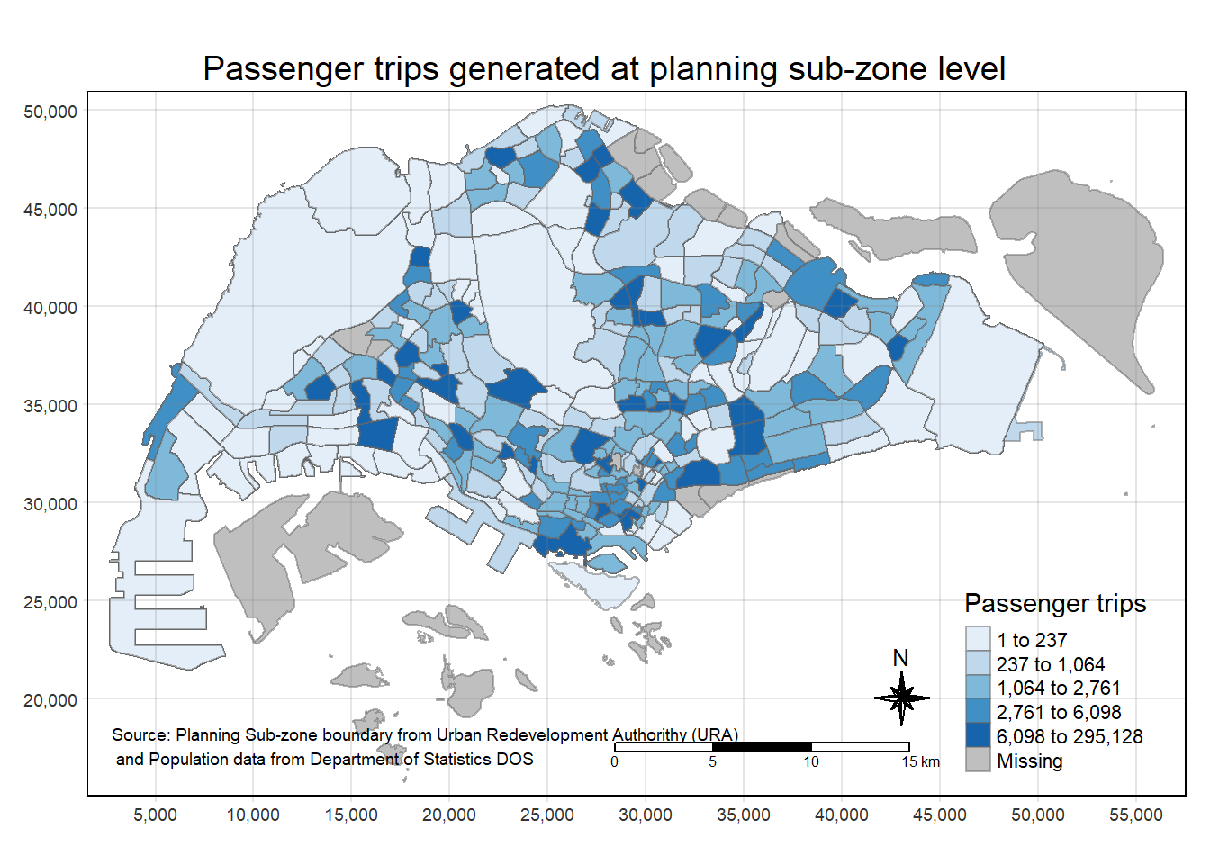
Prepare a choropleth map showing the distribution of passenger trips at planning sub-zone.
tm_shape(mpsz_origtrip)+
  tm_fill("TRIPS",
          style = "quantile",
          palette = "Blues",
          title = "Passenger trips") +
  tm_layout(main.title = "Passenger trips generated at planning sub-zone level",
            main.title.position = "center",
            main.title.size = 1.2,
            legend.height = 0.45,
            legend.width = 0.35,
            frame = TRUE) +
  tm_borders(alpha = 0.5) +
  tm_compass(type="8star", size = 2) +
  tm_scale_bar() +
  tm_grid(alpha =0.2) +
  tm_credits("Source: Planning Sub-zone boundary from Urban Redevelopment Authorithy (URA)\n and Population data from Department of Statistics DOS",
             position = c("left", "bottom"))